The goal of triangulate is to create a generalised version of the bias-adjusted meta-analysis approach originally proposed by Turner et al.
There are a number of steps to this process:
- Define the causal question of interest
- Identify relevant evidence sources and standardise effect directions
- Specify an idealised version of each study
- Assess the extent and direction of bias/indirectness in each result
- Define modifying terms for bias and indirectness in each result
- Calculate bias-/indirectness-adjusted results and perform meta-analysis
This package deals with steps 5 and 6.
⚠️ WARNING NOTES
WARNING #1: This package is under development, and as such the API is subject to change at any point without warning.
WARNING #2: The approach described requires work in the preparation of data to work with the package. Please be sure to read the documentation and make use of helper functions to check whether your data is set-up right.
WARNING #3: The approach described requires careful choice of valid prior distributions of bias/indirectness.
Example
Datasets
The approach described
# Load libraries
library(magrittr)
library(triangulate)

# See column names of dat_bias

colnames(dat_bias)
#>  [1] "result_id" "study"     "type"      "yi"        "vi"        "d1j"
#>  [7] "d1t"       "d1d"       "d2j"       "d2t"       "d2d"       "d3j"
#> [13] "d3t"       "d3d"       "d4j"       "d4t"       "d4d"       "d5j"
#> [19] "d5t"       "d5d"       "d6j"       "d6t"       "d6d"       "d7j"
#> [25] "d7t"       "d7d"

head(dat_bias)
#>   result_id   study type          yi         vi      d1j d1t
#> 1   13401-2 Study 1 NRSI -0.12783337 0.12506586     High Add
#> 2   14632-2 Study 2 NRSI -0.19845094 0.08680919 Moderate Add
#> 3   14658-2 Study 3 NRSI -0.18632958 0.03361240     High Add
#> 4   14665-6 Study 4 NRSI  0.19062036 0.05526578     High Add
#> 5   14720-1 Study 5 NRSI -0.56211892 0.05141924     High Add
#> 6   14761-1 Study 6 NRSI -0.09431068 0.06969822     High Add
#>                    d1d      d2j  d2t                d2d      d3j  d3t
#> 1   Favours comparator      Low None               None Moderate Prop
#> 2 Favours experimental Moderate  Add Favours comparator      Low None
#> 3   Favours comparator     High  Add Favours comparator      Low None
#> 4   Favours comparator Moderate  Add      Unpredictable      Low None
#> 5   Favours comparator      Low None               None      Low None
#> 6   Favours comparator Moderate  Add Favours comparator      Low None
#>             d3d d4j  d4t  d4d      d5j  d5t           d5d      d6j  d6t
#> 1 Unpredictable Low None None      Low None          None      Low None
#> 2          None Low None None      Low None          None Moderate  Add
#> 3          None Low None None      Low None          None Moderate  Add
#> 4          None Low None None      Low None          None      Low None
#> 5          None Low None None Moderate Prop Unpredictable      Low None
#> 6          None Low None None Moderate Prop Unpredictable      Low None
#>             d6d      d7j  d7t            d7d
#> 1          None Moderate Prop Away from null
#> 2 Unpredictable Moderate Prop Away from null
#> 3 Unpredictable Moderate Prop Away from null
#> 4          None Moderate Prop Away from null
#> 5          None Moderate Prop Away from null
#> 6          None Moderate Prop Away from null

tri_dat_check(dat_bias)
#> Looks good!
#> All expected columns are present in the dataset.
For details on how to create these datasets, see the Creating triangulation datasets vignette (under construction).
Once we load our data, helper functions will convert it to long format and convert to absolute directions of bias/indirectness.
dat_bias <- triangulate::dat_bias %>%

# Convert to long format
tri_to_long() %>%

tri_absolute_direction() %>%

tri_append_bias(triangulate::dat_bias_values)
Then apply the same approach to the indirectness dataset:
dat_ind <- triangulate::dat_ind %>%
# Convert to long format
tri_to_long() %>%
tri_absolute_direction() %>%
tri_append_indirect(triangulate::dat_ind_values)
Add prior distributions of bias/indirectness
dat_bias_values
#>   domain        j bias_m_add bias_v_add bias_m_prop bias_v_prop
#> 1    all     high       0.18       0.10        0.06       0.032
#> 2    all moderate       0.09       0.05        0.03       0.016
#> 3    all      low       0.00       0.00        0.00       0.000
Create final dataset and analyse
We now have two clean datasets, one for bias and one for indirectness, that we can use to
dat_final <- tri_prep_data(dat_bias, dat_ind)
#> Joining with `by = join_by(result_id)`
#> Joining with `by = join_by(result_id)`
#> Joining with `by = join_by(result_id)`
#> Joining with `by = join_by(result_id)`
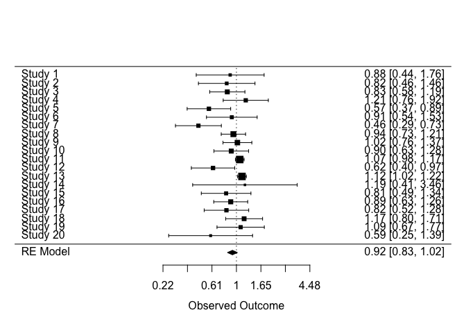
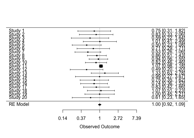
At this point, we have an unadjusted (yi, vi) and adjusted (yi_adj, vi_adj) estimates for each result.
These estimates can then simply be passed to metafor for analysis
model <- metafor::rma(
  yi = yi,
  vi = vi,
  data = dat_final,
  slab = dat_final$study,
  method = 'DL'
)

# Pass model to forest plot function
metafor::forest(
  model,
  atransf = exp,
)
model_adj <- metafor::rma(
  yi = yi_adj,
  vi = vi_adj,
  data = dat_final,
  slab = dat_final$study,
  method = 'DL'
)

# Pass model to forest plot function
metafor::forest(
  model_adj,
  atransf = exp
)